Module 7: Autocorrelation Function Estimation

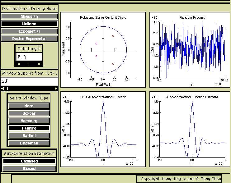
Explanation:
Let x(n) be a linear random process generated by passing a zero-mean, i.i.d., unit variance process w(n) through a linear filter with impulse response h(n). The autocorrelation function of x(n) is defined as r(k)=E[x(n) x(n+k)] and is related to the system impulse response through r(k)=sum_n h(n) h(n+k). If x(n) is real and stationary, then r(k)=r(-k).

Given N samples of x(n), we estimate r(k) by averaging the product x(n) x(n+k) over all available n's at lag k. The total number of such terms is N-|k|. The unbiased estimate is then the running sum of x(n) x(n+k) divided by N-|k|, whereas for the biased estimate, the divisor is N.

Because there are fewer number of terms to average at larger lags, the r(k) estimate is less reliable at larger |k|. To compensate for this, we taper the r(k) estimate by multiplying the sample r(k) with a window function w(k) which is symmetric and monotonically non-increasing with |k|.

To use this applet, first select the poles and zeros of the system. Once the system is defined, theoretical autocorrelation function can be calculated as shown in the lower left panel of the applet. Next, choose the probability distribution function (pdf) for the driving noise w(n), as well as the data length N. A realization of w(n) is then plotted in the top right panel. Without windowing and especially with the unbiased option, the sample autocorrelation function is inaccurate at larger lags. Toggle between the biased and unbiased options, we see that the difference between the two is more noticeable at larger values of |k|. Use a tapering windows and adjust its parameter L to improve the autocorrelation function estimate. If we know a priori that the system impulse response has no more than L points, or the memory of the process is no more than L, then a length L window should be used.

Observe the following:

• The theoretical autocorrelation function does not depend on the pdf of the driving noise.
• At a fixed lag, the longer the data length, the more accurate the sample autocorrelation estimate.
• Windowing improves the autocorrelation function estimate.

Experiment it yourself!
Click here to run the experiment using your browser.

Instruction: To change a parameter from its default value, slide the bar beneath the parameter window or enter a specific number and then hit the return key. Hitting the return key from any of the parameter windows initiates another Monte Carlo run.