Module 4: The Central Limit Theorem

Explanation:
The Central Limit Theorem: Suppose that Xi are independent, identically distributed r.v.'s with mean m and finite variance s^2, and denote the sum of n such r.v.'s as Sn=(X1+X2+...+Xn). Let Zn be the standardized version of Sn; i.e., Zn=(Sn-nm)/(sqrt(n)s), then as n goes to infinity, Zn tends to the standard Gaussian distribution (i.e., with mean 0 and variance 1). This is true regardless of the distribution of Xi. Implication: for n large, the sample mean, mX=(X1+X2+...+Xn)/n, is approximately Gaussian distributed with mean m.

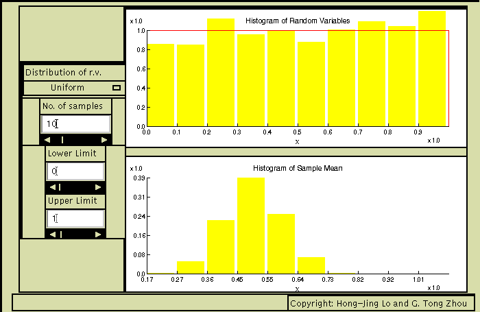
To use this applet, we first select the pdf of Xi from the Distribution of r.v. menu (default=Gaussian). Next, set the corresponding distribution parameters and the number of samples n (default=10). Random variables X1, X2, ..., Xn that have the chosen pdf are then generated. The top window shows the normalized histogram (estimated pdf) of Xi in yellow and the selected pdf in red. Normalized histogram of the sample mean mX is shown in the bottom window. For a "large" n (for example n=10 ), it can be seen that no matter what pdf Xi has, the histogram of the sample mean mX always tends to be Gaussian-shaped. For a pdf of Xi other than Gaussian, we observe that as we gradually slide the No. of samples bar to the right (i.e., slowly increasing n ), the estimated pdf becomes more and more bell-shaped. If Xi is Gaussian, then the sample mean is always Gaussian regardless of what n we use.

Experiment it yourself!
Click here to run the experiment using your browser.

Instruction: To change a parameter from its default value, slide the bar beneath the parameter window or enter a specific number and then hit the return key. Hitting the return key from any of the parameter windows initiates another Monte Carlo run.